timeline
    title R Workshop Series 2025
    May 14-15  : Beginner Workshop (2 days)
    Sep 18-19 : Intermediate Workshop (2 days)
    Nov 20-21 : Advanced Workshop (2 days)
R Beginners Course 2025
Introduction to R and Basic Programming Concepts
2025-05-13
Welcome to the R Workshop Series!

- Learning R step-by-step
Welcome to the R Workshop Series!
- Learning R step-by-step
- Focus: Molecular Biology and Data Analysis
Welcome to the R Workshop Series!
- Learning R step-by-step
- Focus: Molecular Biology and Data Analysis
- Building reproducible research skills (at data level)
Workshop Goals
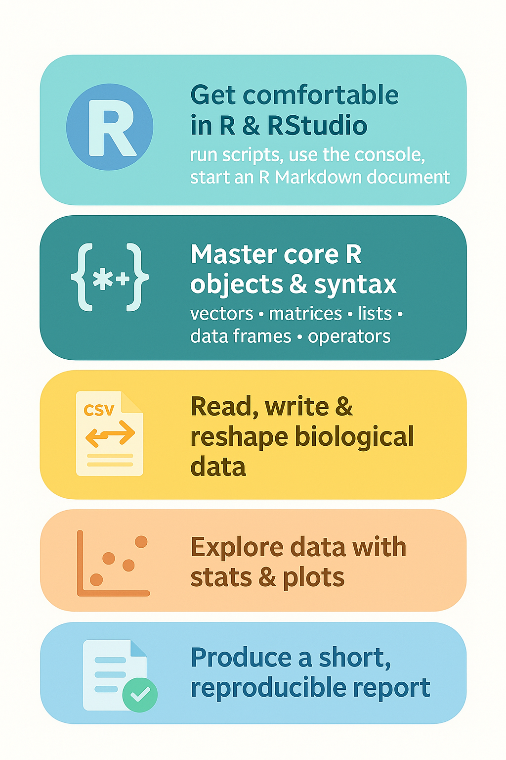
Five Goals
Learning Between Workshops
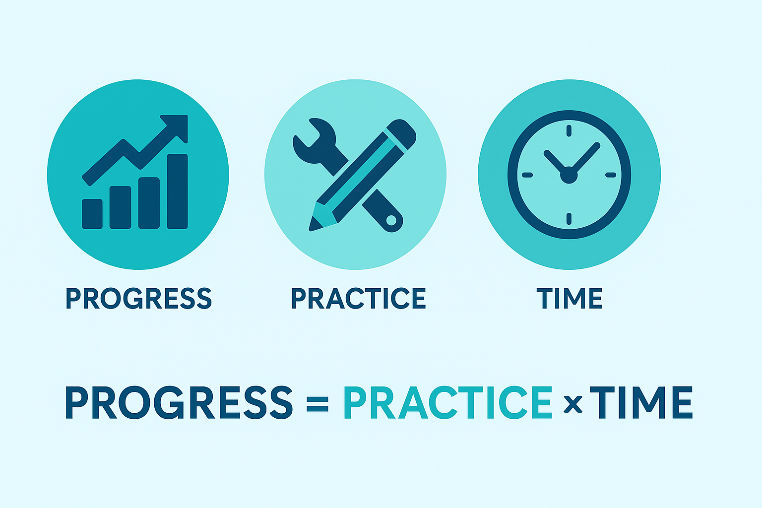
Learning Between Workshops
- Learning R = Learning a language: Use it often!
Learning Between Workshops
- Learning R = Learning a language: Use it often!
- Practice exercises, small projects
Learning Between Workshops
- Learning R = Learning a language: Use it often!
- Practice exercises, small projects
- Apply R to your own data
Learning Between Workshops
- Learning R = Learning a language: Use it often!
- Practice exercises, small projects
- Apply R to your own data
- Prepare questions for next workshop
Slides & Code

- [f] Full screen
- [o] Slide Overview
- [c] Notes
- [h] help
git repo
Clone repo
git clone https://github.com/CECADBioinformaticsCoreFacility/Beginners_R_Course_2025.git
Slides Directly
https://cecadbioinformaticscorefacility.github.io/Beginners_R_Course_2025/
The Lifeline of R
The Lifeline of R
- R was born as an implementation of S in 1993, because
native S had gone commercial - Being free and encouraging contributions by the user community,
R can easily "evolve" to adapt to new needs and trends Data driven science, including the genome projects, was the perfect “niche” which R could successfully claim for itself- Indeed the
Bioconductor projectwas initiated by one of the founders of R
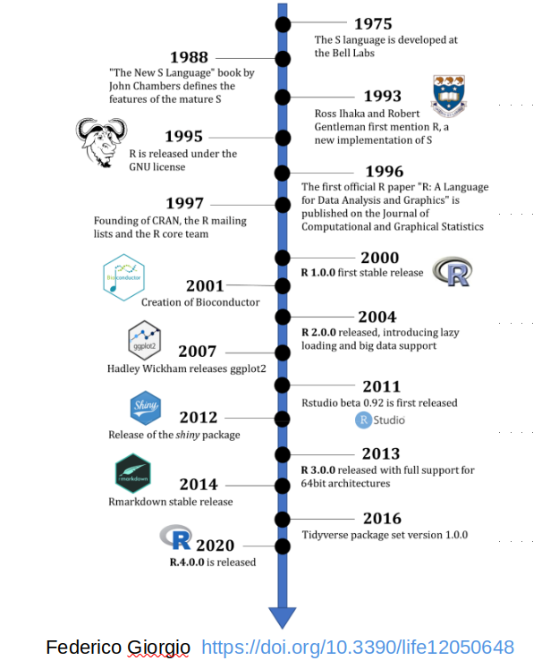
The Lifeline of R
- The
RStudio (now: Posit)company is gaining increasing influence on the evolution of the language- its
Integrated Development Environment (IDE)is increasingly used by people doing data analysis with R - Posit is actively developing and promoting the
tidyverse, which is both a special style and a code repository for the analysis ofdata tables
- its
- Currently there is quite some
evolutionary pressurefor change of the language!
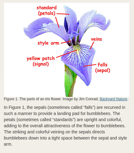
The Iris Data of Edgar Anderson and Ronald A. Fisher
– Some Background Information on Our Practice Dataset
We will use the iris dataset of floral traits for practicing throughout the course:
The Iris Data of Edgar Anderson and Ronald A. Fisher
– Some Background Information on Our Practice Dataset
- Data published by Ronald A. Fisher in 1936
- Statistician and co-founder of population genetics
- Plants collected by Edgar Anderson
- I. setosa and I. versicolor in 1935,
in the same natural habitat - I. virginica likely in 1926,
at a different place
- I. setosa and I. versicolor in 1935,
- Field botanist with a focus on speciation mechanisms
The Iris Data of Edgar Anderson and Ronald A. Fisher
– Some Background Information on Our Practice Dataset
Both men were involved in the making of the Modern/Evolutionary Synthesis, with complementary central tenets:
- R. A. Fisher: Model evolutionary processes from the known facts of genetics
- E. Anderson: Observe the real dynamics of (plant) populations, in order to understand the role of genetics in evolution
The Iris Data of Edgar Anderson and Ronald A. Fisher
– Some Background Information on Our Practice Dataset
Edgar Anderson suspected that I. versicolor may be an allopolyploid hybrid:
I. versicolor =
I. setosa (2n) x I. virginica (4n)
(confirmed by Lim et al. 2007)This may have supported the establishment of the species, by preventing back-crossing to its parents.
Fisher applied his Linear Discriminant Analysis technique to Anderson’s data, in order to test the hypothesis of additive gene action:
if true, versicolor should be twice as similar to virginica than to sertosa!
Interacting R
Variables
- Variables are containers for storing data values.
- R does not have a command for declaring a variable
- A variable is created the moment you first assign a value to it.
- Assignment operator
<-/=can be used for assigning a value
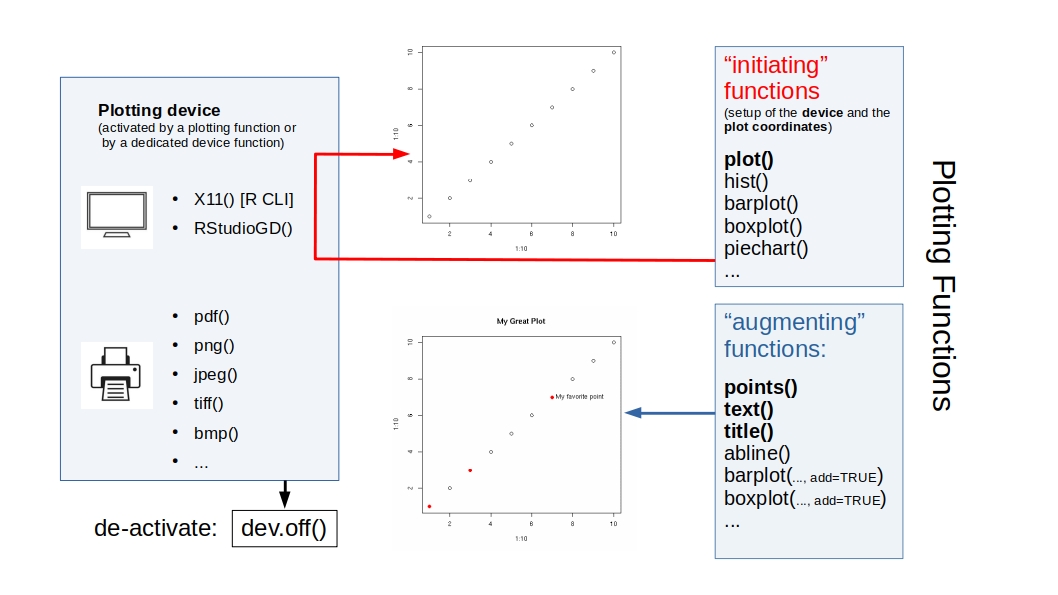
R Plots (base)
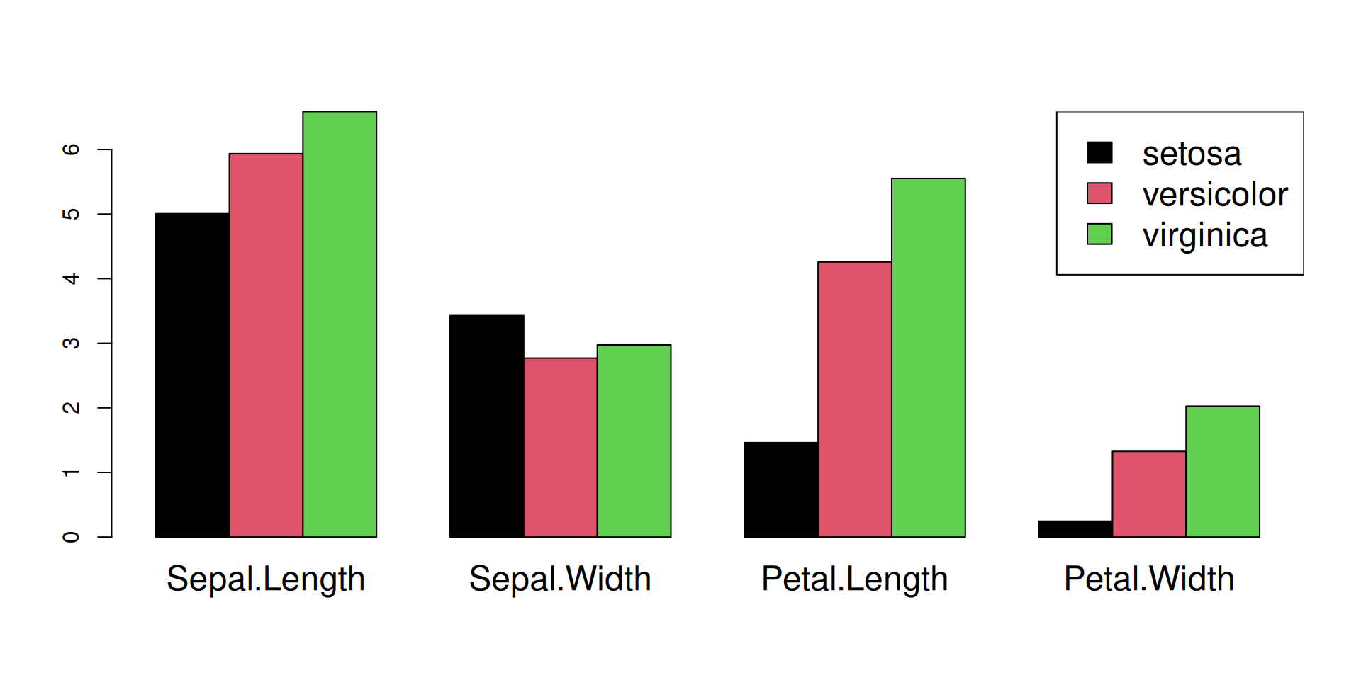
R Plots (base) – barplot()
Barplots represent sign and absolute value of numbers by the direction and length of bars.
If called with a matrix as first argument, the function produces one plot for each column:
R Plots (base) – barplot()
If we want to plot trait means per species, we must change the rows of matrix species_means (= the species) into columns, because barplot() reads a matrix by column.
This is done by the t() function ("transpose"):
m <-  t(species_means) ## TRANSPOSE

barplot(## one plot per column == species,
        ## one bar == trait mean!
        m,

        ## do not stack the bars
        beside=TRUE,

        ## larger group labels
        cex.names=2,

        col=trait_colors,

        ## increase y limit to fit the legend
        ylim = c(0,10),
        cex = 2
        )

## add a legend (plot "augmentation"!)
legend(x=1,y=10, ##"topright",
       rownames(m),
       fill=trait_colors)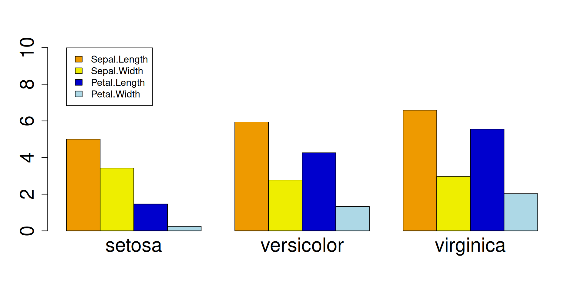
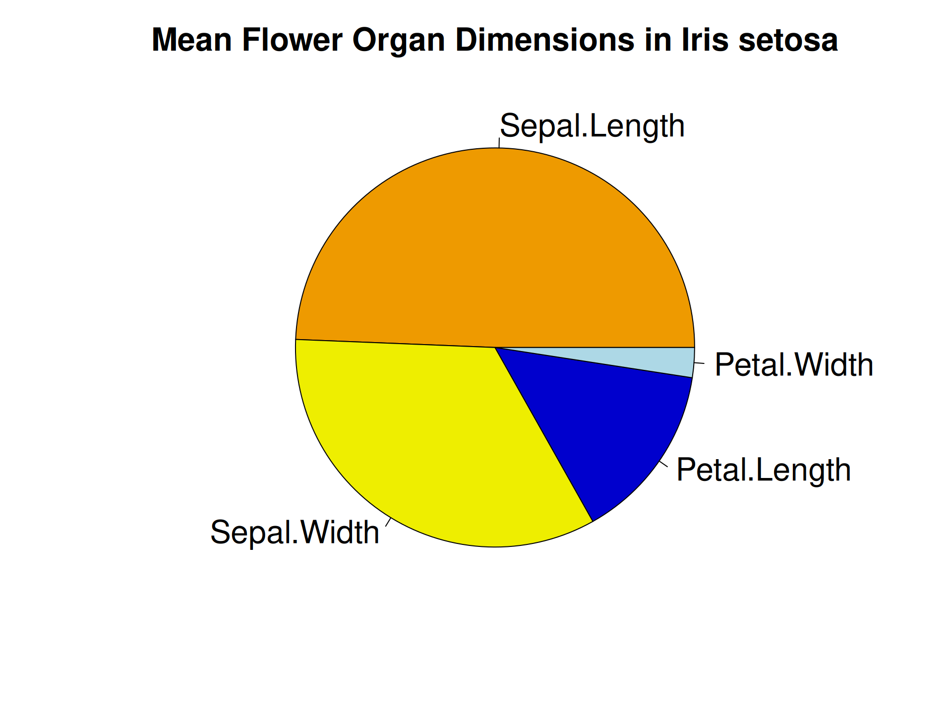
R Plots (base) – pie()
Piecharts are a quick-and-dirty alternative for representing numbers.
The pie() function can only represent one set of numbers at a time. In addition, comparing angles on a piechart is visually not as easy as comparing bar heights.
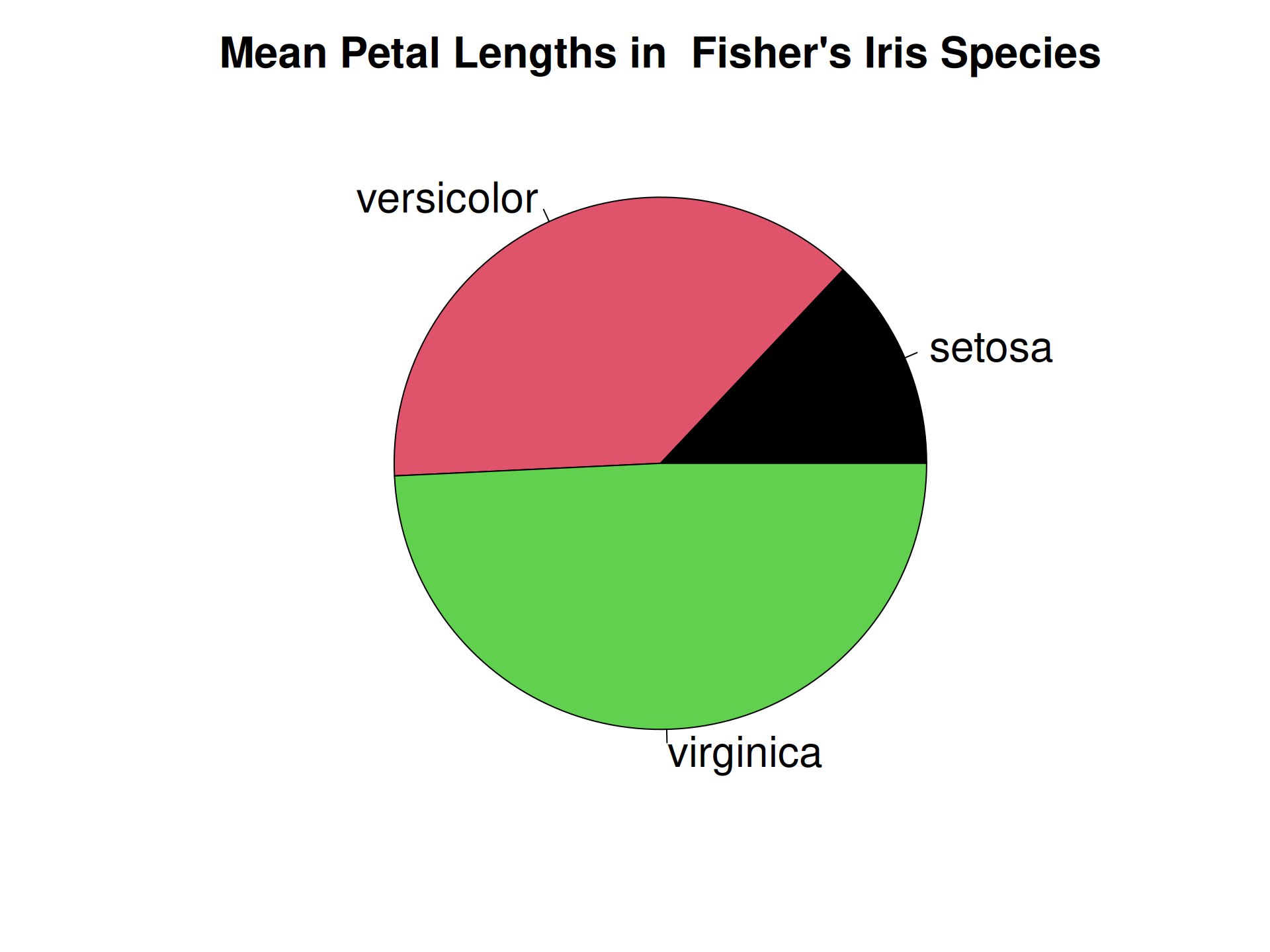
R Plots (base) – pie()
Piecharts are a quick-and-dirty alternative for representing numbers.
The pie() function can only represent one set of numbers at a time. In addition, comparing angles on a piechart is visually not as easy as comparing bar heights.
R Plots (base) – plot()
The plot() function is an extremely versatile workhorse for x/y plots.
As an “initializing” function, it may be called to just create an empty canvas, to be filled later:
R Plots (base) – plot()
Or it is called with an initial set of data, with the option to extend the plot later:
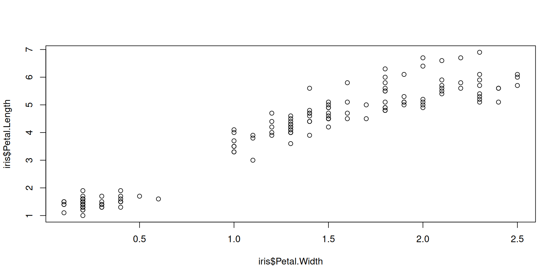
R Plots (base) – plot()

R Plots (base) – plot()

R Plots (base) – plot()
Overplot some points with color, in order to identify a group in your data:
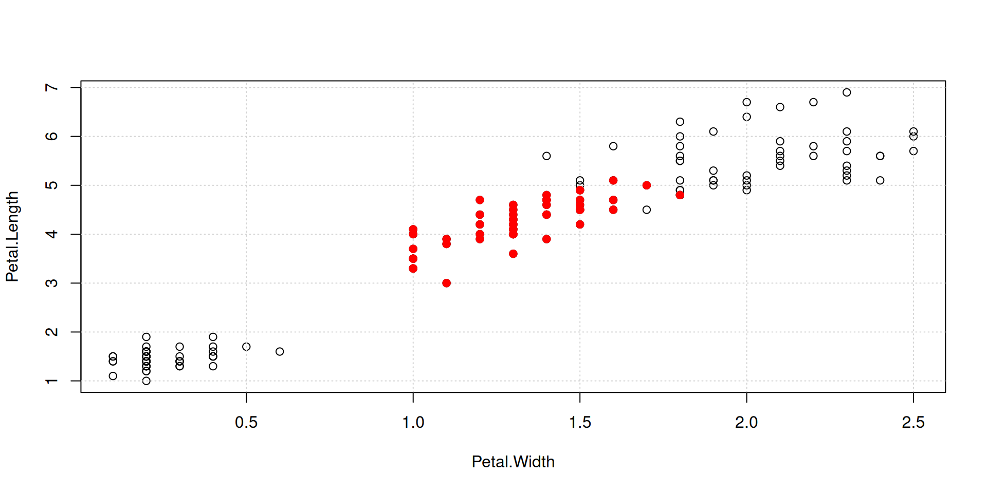
R Plots (base) – plot()
Color all points by species, using our named vector species_colors:
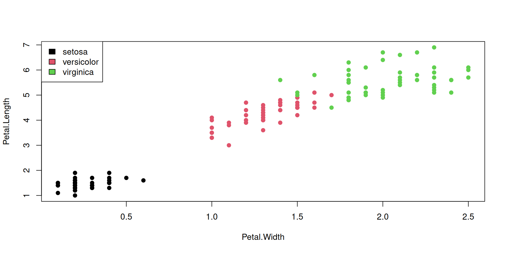
R Plots (base) – plot()
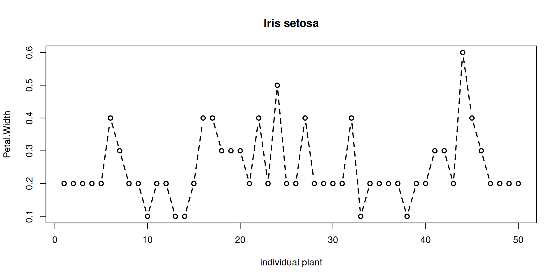
Points with adjacent positions in the input can be connected by lines, using different line styles. A typical use case is a line graph, with x as a running number or ID.
## See par() for line-related parameters!

## Make a new data.frame,
## containing only setosa:
df <- subset(iris, Species=="setosa")

plot(
     # x is now the row number in df
     x=1:nrow(df),
     xlab="individual plant",

     y=df$Petal.Width,
     ylab="Petal.Width",

     ## show both points and
     ## connecting lines:
     type="b",

     ## line width:
     lwd = 2,
     ## line style = dashed:
     lty=2,

     main="Iris setosa"
)
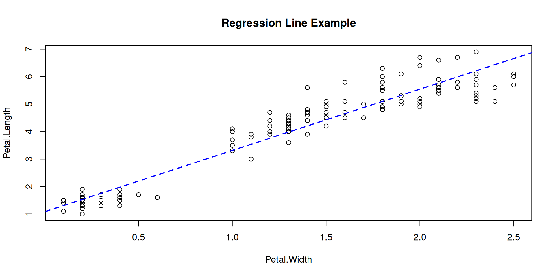
R Plots (base) – plot()
It can make sense to connect some points in a general scatterplot by lines.
The augmenting function lines() can do this.
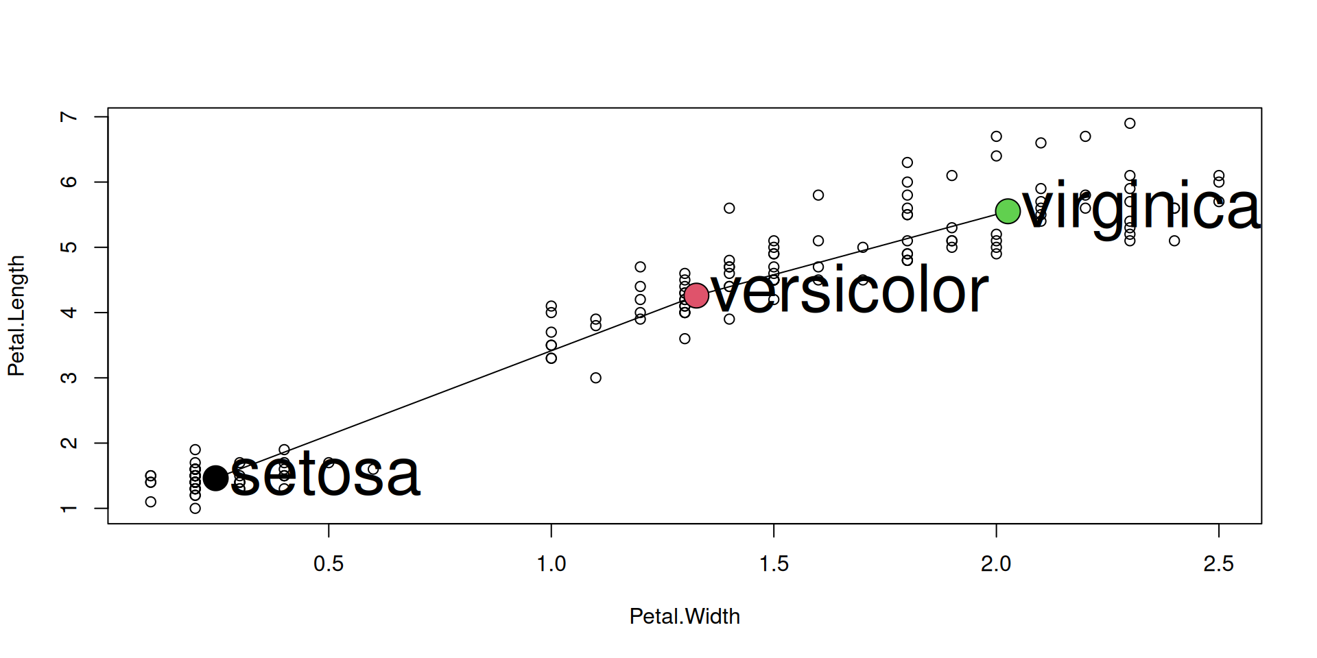
Here, we want to connect the (x,y) means of our three species:
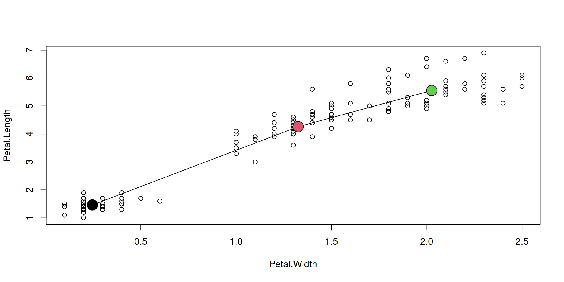
R Plots (base) – plot()
Annotate individual points:
R Plots (base) – plot()
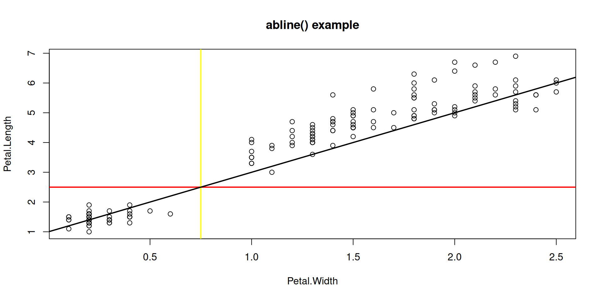
Function abline() adds indicator lines to a plot.
R Plots (base) – plot()
Function abline() adds indicator lines to a plot.
Lines marking locations or slopes of interest:
R Plots (base) – layout()
layout(m) ## read the layout matrix

use_cols =  species_colors[iris$Species]
## 1
plot(Sepal.Length ~ Sepal.Width, data=iris,
     pch=21, col=use_cols, bg=use_cols,
     cex.lab=2)
## 2
plot(Petal.Length ~ Petal.Width, data=iris,
     pch=21, col=use_cols, bg=use_cols,
     cex.lab=2)
## 3
plot(Sepal.Length ~ Petal.Length, data=iris,
     pch=21, col=use_cols, bg=use_cols,
     cex.lab=2)
## 4
plot(Sepal.Width ~ Petal.Width, data=iris,
     pch=21, col=use_cols, bg=use_cols,
     cex.lab=2)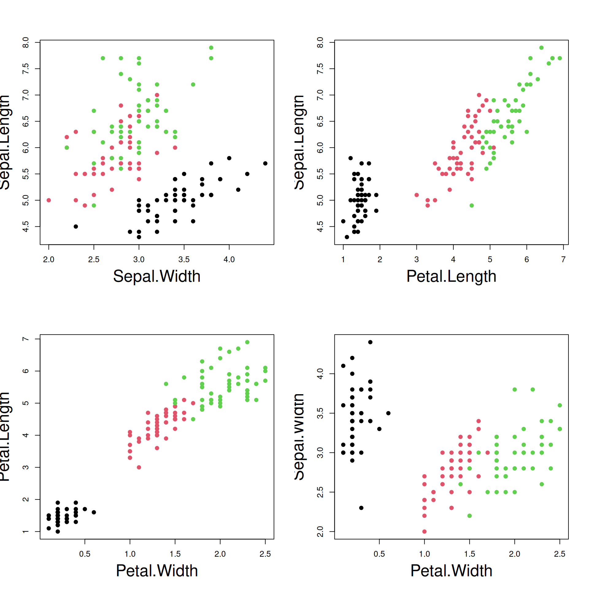
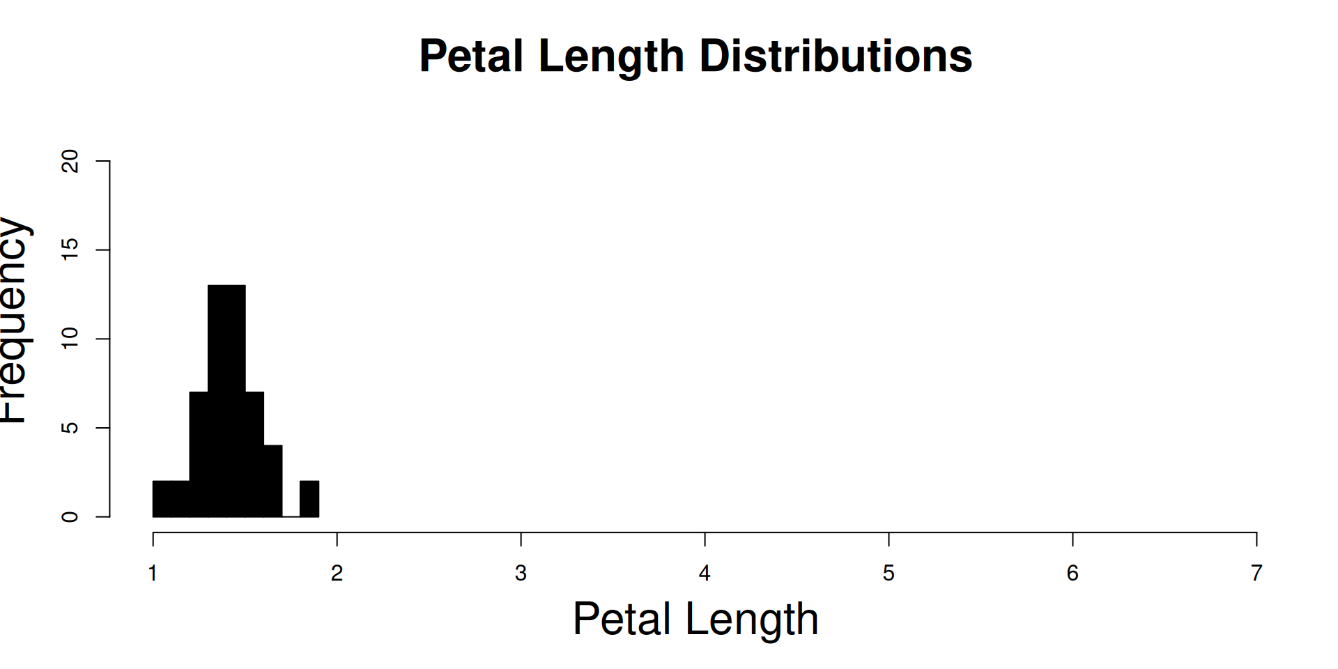
R Plots (base) – hist()
The hist() function is one of those “dual use functions”:
With add=FALSE, it initializes the device and the coordinate system, while
with add=TRUE, its output goes directly to an existing plot.
setosa <- subset(iris,Species=="setosa")
versicolor <- subset(iris,Species=="versicolor")
virginica <- subset(iris,Species=="virginica")

## Plot the histogram of setosa,
## and initialize the entire plot:

hist(setosa$Petal.Length,
     col=species_colors["setosa"],

     add=FALSE, ## this is the default

     ## initialize to full x range !
     xlim=range(iris$Petal.Length),

     ## full y range you usually
     ## only know after some trials ..
     ylim=c(0,22),

     ## x-axis label
     xlab="Petal Length",

     ## larger axis labels:
     cex.lab = 2,

     main = "Petal Length Distributions",

     ## larger title:
     cex.main = 2
)
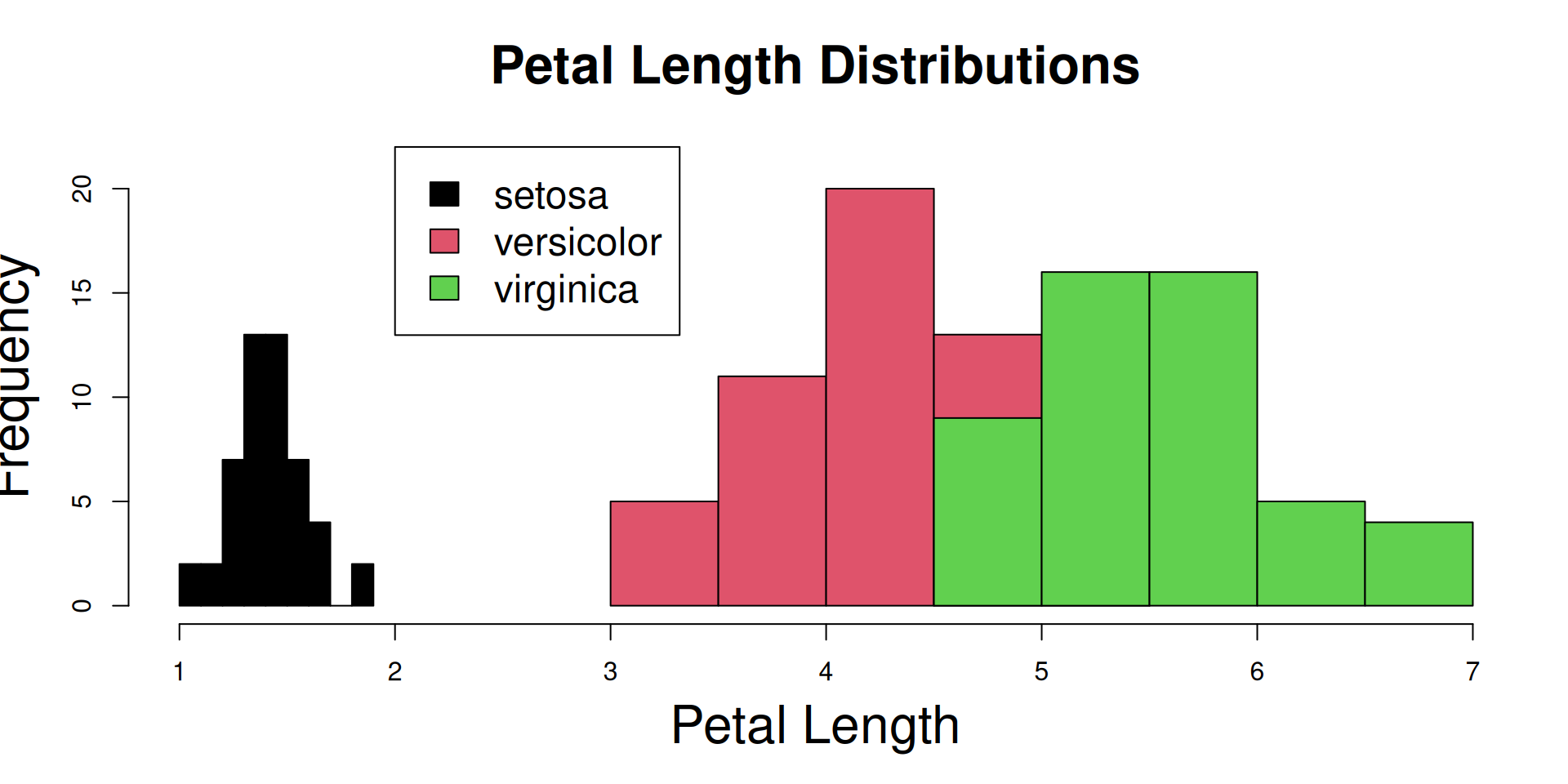
R Plots (base) – hist()
The hist() function is one of those “dual use functions”:
With add=FALSE, it initializes the device and the coordinate system, while
with add=TRUE, its output goes directly to an existing plot.
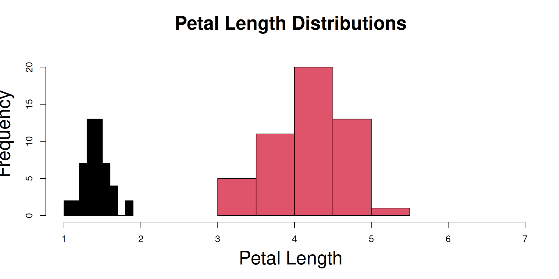
R Plots (base) – hist()
The hist() function is one of those “dual use functions”:
With add=FALSE, it initializes the device and the coordinate system, while
with add=TRUE, its output goes directly to an existing plot.
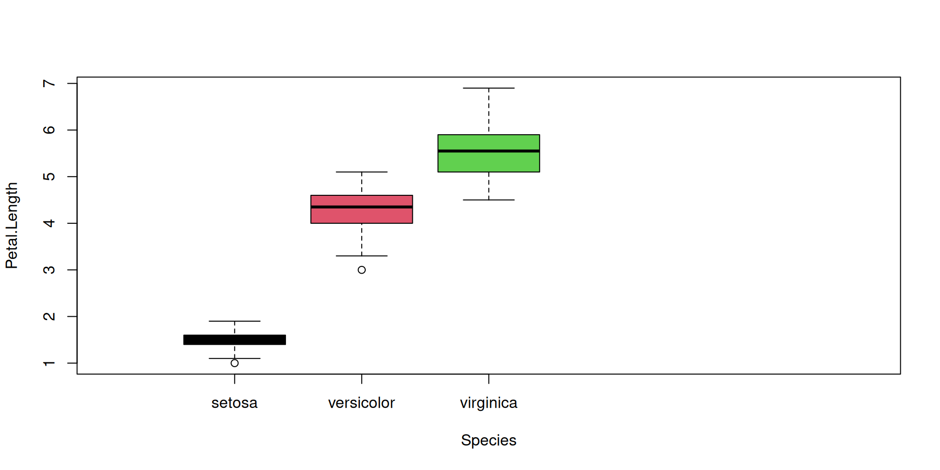
R Plots (base) – boxplot()
The boxplot() function has “dual-use” capabilities, too.
However it can accept a formula with a factor on the right hand side, and it will split the dataset automatically according to the factor levels. So we can plot all species at once:
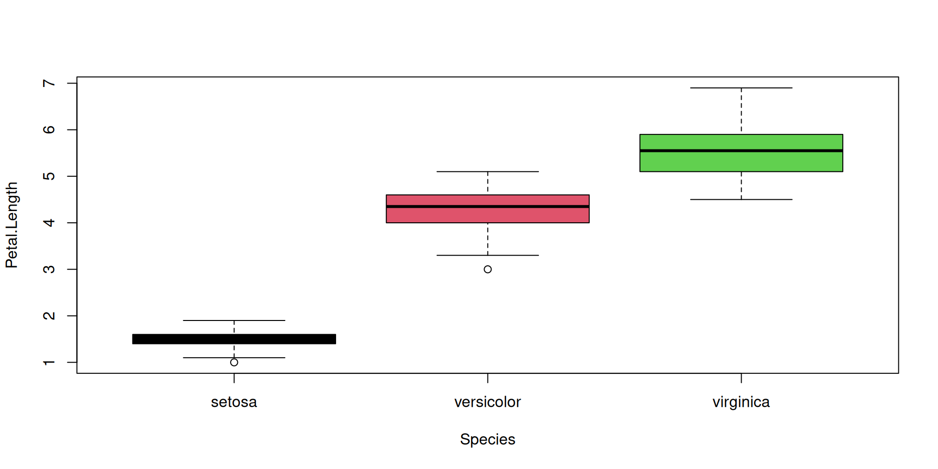
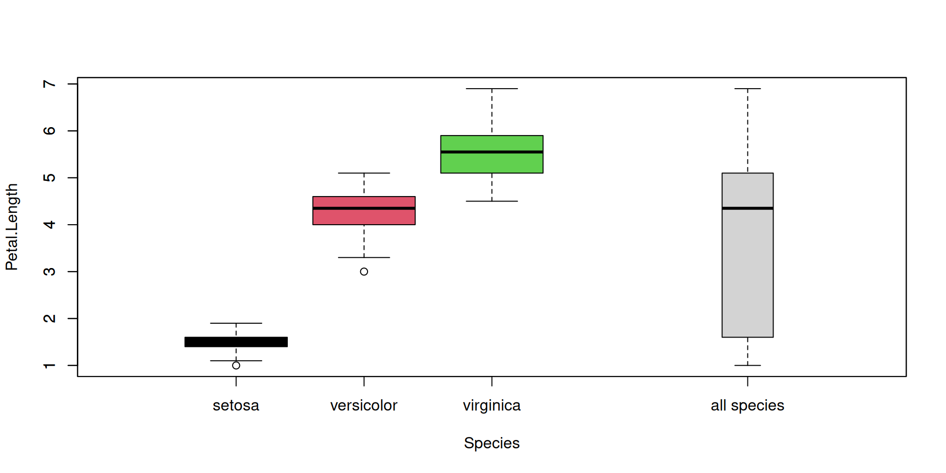
R Plots (base) – boxplot()
Let’s add a boxplot for the global Petal.Length distribution (all species merged):
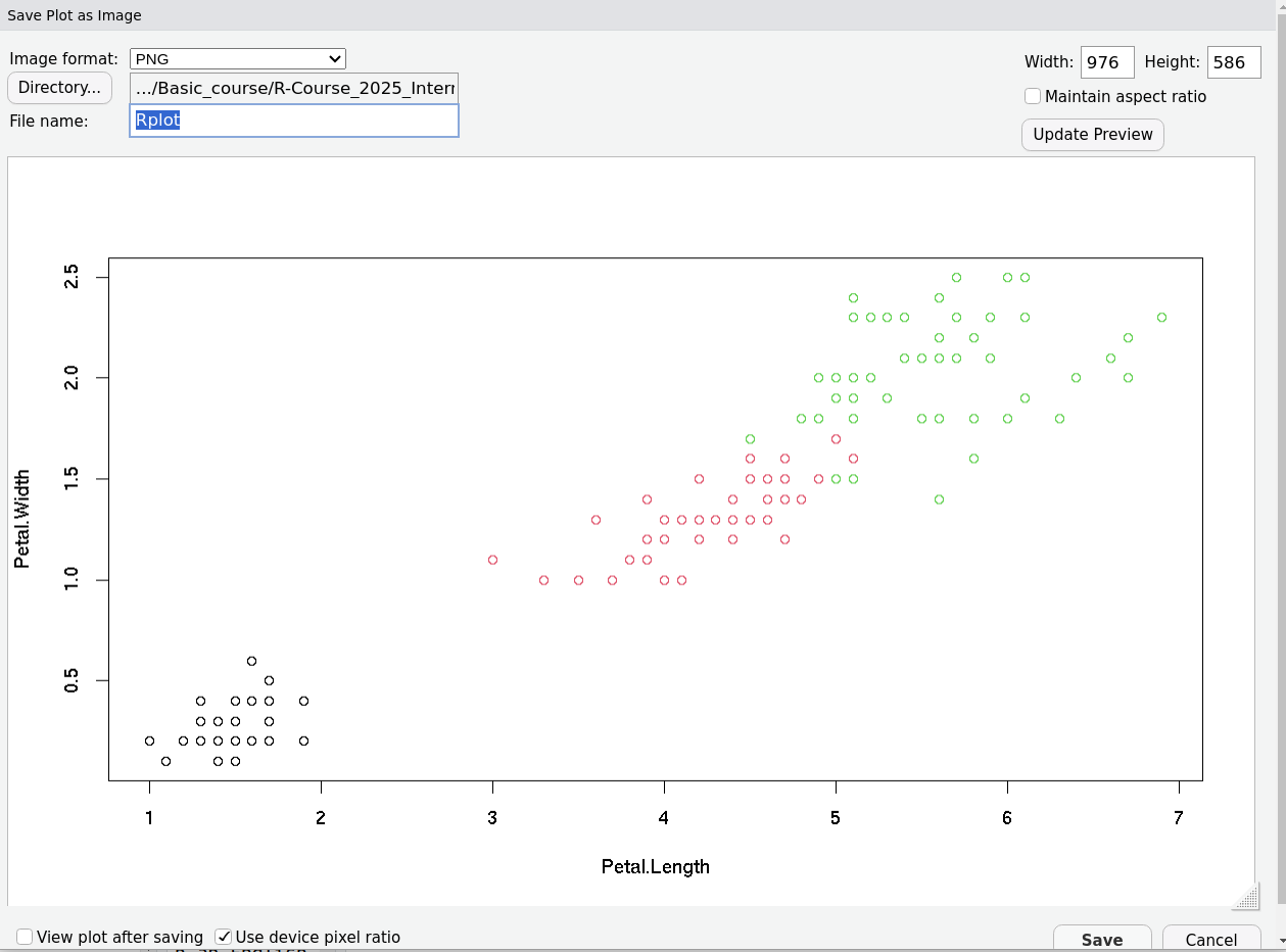
R Plots (base) – Saving Plots From RStudio
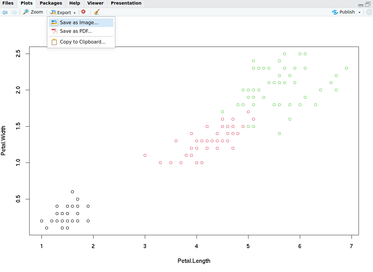
R Plots (base) – Saving Plots From RStudio
Digression: Software is Usually Built From Bits and Pieces
- … they come under the names of subroutines, macros, functions …
- … in code, they are used like ’commands’:
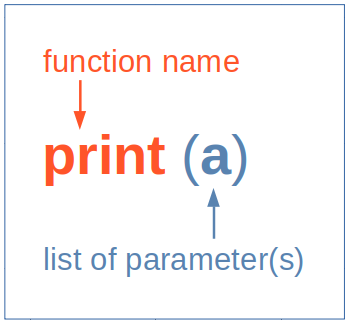
- Actually the function name invokes a piece of hidden code
- … hiding complexity
- … yet allowing to easily access complex algorithms
- … and to make local extensions of a language
![]()