
R Beginners Course 2025
Introduction to R and Basic Programming Concepts
2025-03-17
Measures of Central Tendency
mean, median, mode
  3 2.8 3.2 3.4 3.1 2.9 2.7 2.5 3.3 3.5 3.8 2.6 2.3 3.6 2.2 2.4 3.7 3.9   2   4
 26  14  13  12  11  10   9   8   6   6   6   5   4   4   3   3   3   2   1   1
4.1 4.2 4.4
1 1 1 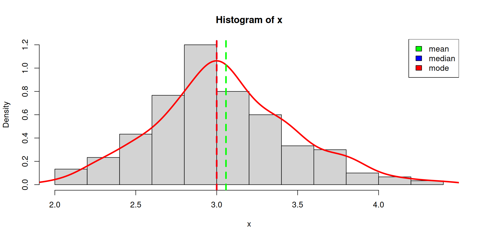
Measures of Variability
Min, max, range

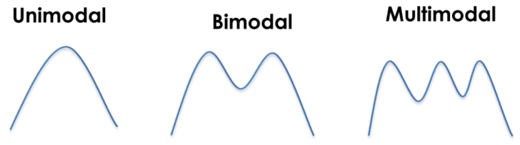
Measures of Distribution
Modes
The modality of a distribution is determined by the number of peaks it contains
Skewness
Skewness is a measurement of the symmetry of a distribution.
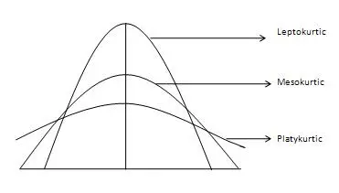
Kurtosis
Kurtosis measures whether your dataset is heavy-tailed or light-tailed compared to a normal distribution.

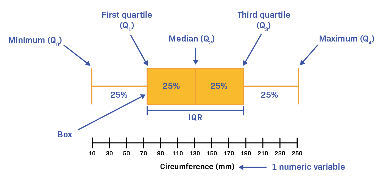
Descriptive Statistics
  Sepal.Length    Sepal.Width     Petal.Length    Petal.Width
 Min.   :4.300   Min.   :2.000   Min.   :1.000   Min.   :0.100
 1st Qu.:5.100   1st Qu.:2.800   1st Qu.:1.600   1st Qu.:0.300
 Median :5.800   Median :3.000   Median :4.350   Median :1.300
 Mean   :5.843   Mean   :3.057   Mean   :3.758   Mean   :1.199
 3rd Qu.:6.400   3rd Qu.:3.300   3rd Qu.:5.100   3rd Qu.:1.800
 Max.   :7.900   Max.   :4.400   Max.   :6.900   Max.   :2.500
       Species
 setosa    :50
 versicolor:50
 virginica :50
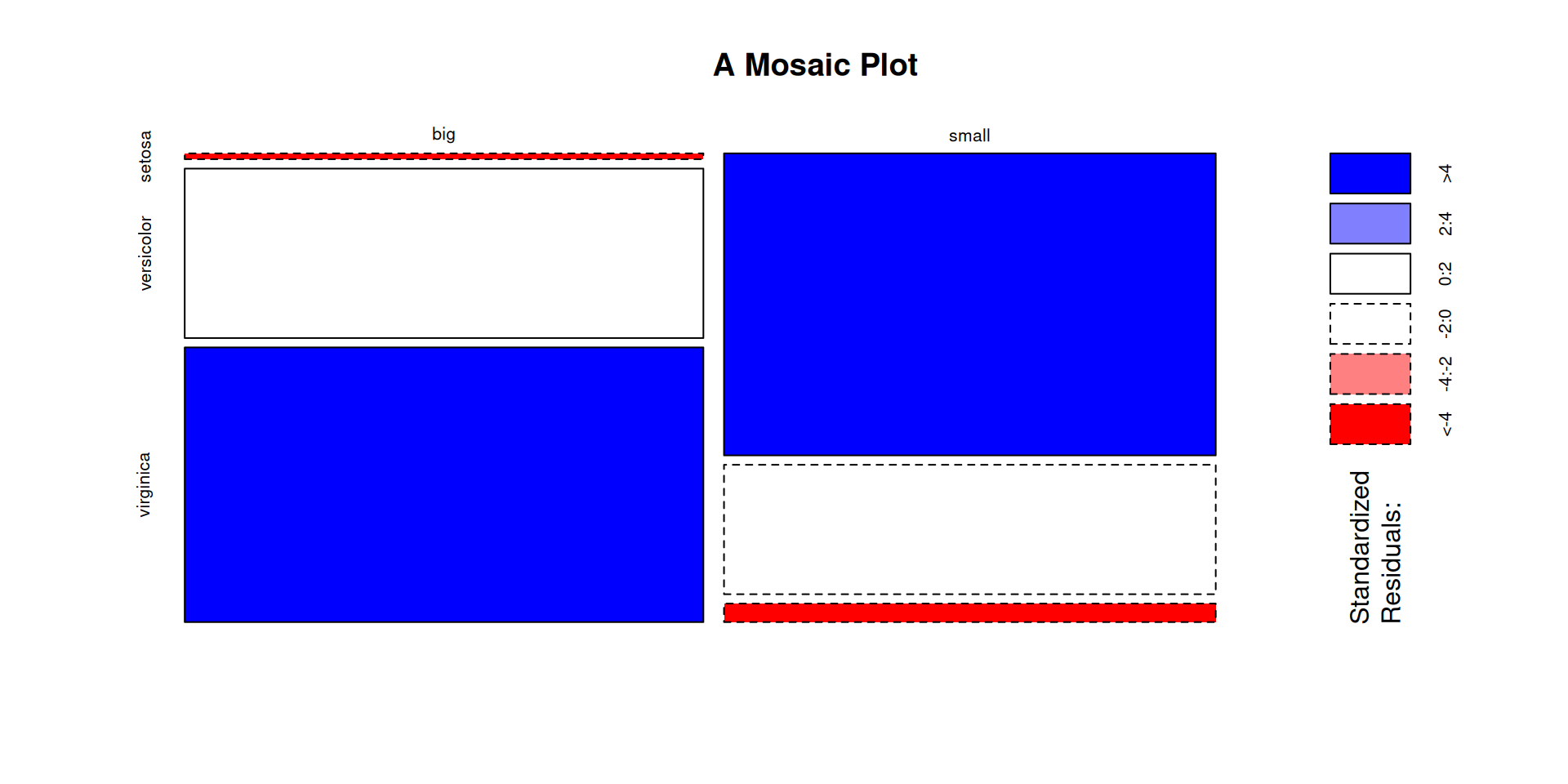
Frequency/Cross/Contingency Tables
Cross-tabulation analysis, also known as contingency table analysis, is most often used to analyze categorical (nominal measurement scale) data.
At their core, cross-tabulations are simply data tables that present the results of the entire group of respondents, as well as results from subgroups of survey respondents. With them, you can examine relationships within the data that might not be readily apparent when only looking at total survey responses
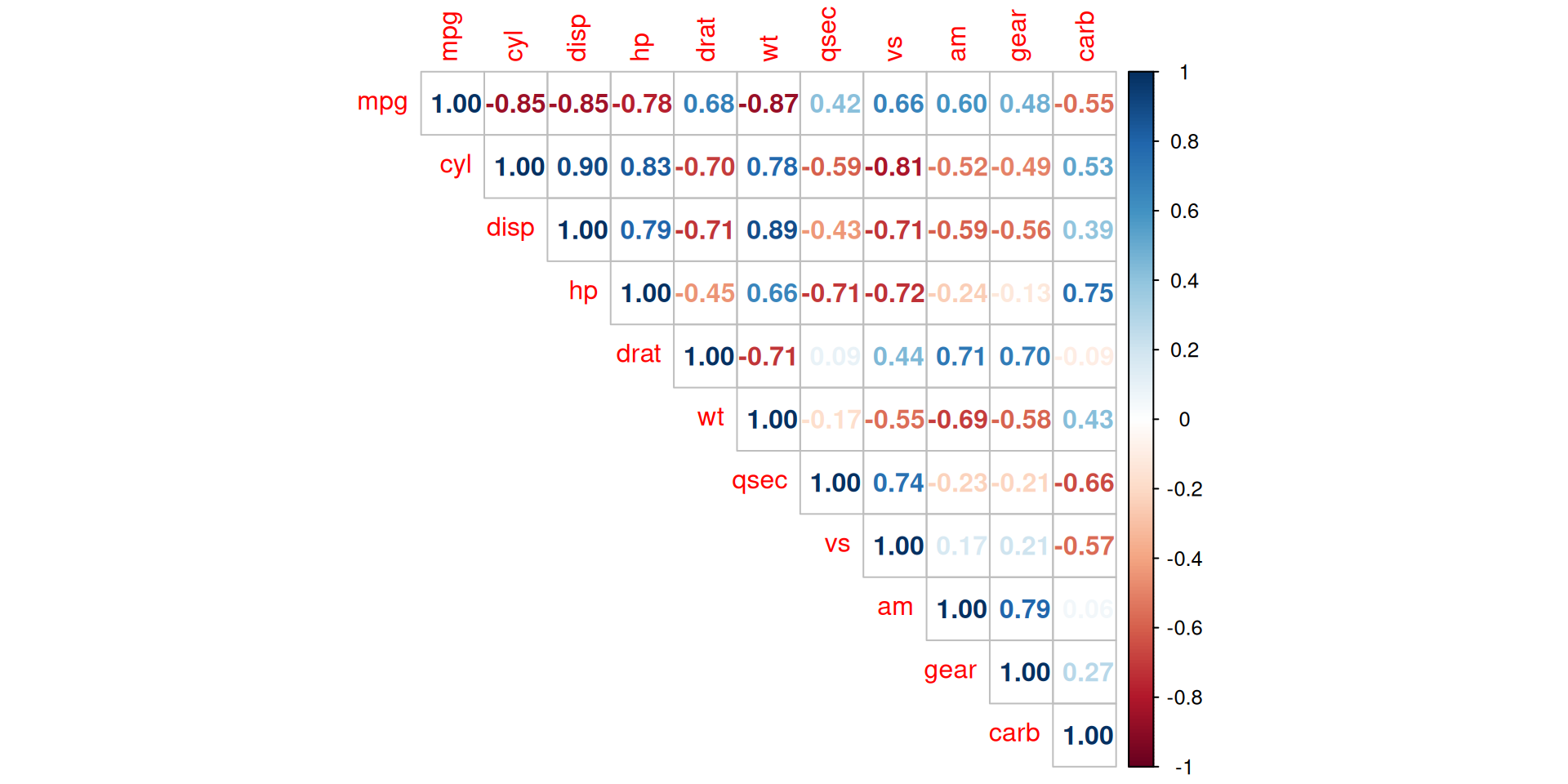
Correlation
Correlation measures the relationship between two variables if they are linked to each other. It denotes if variables evolve in the same direction, in the opposite direction, or are independent.
Correlation is usually computed on two quantitative variables, but it can also be computed on two qualitative ordinal variables.
Pearson correlation is often used for quantitative continuous variables that have a linear relationship
Spearman correlation (which is actually similar to Pearson but based on the ranked values for each variable rather than on the raw data) is often used to evaluate relationships involving at least one qualitative ordinal variable or two quantitative variables if the link is partially linear
R Loops
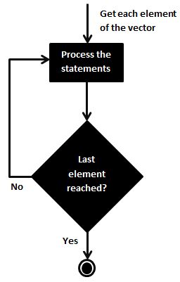
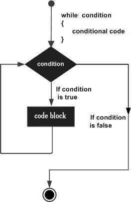
Practice 2
- Use
forand/orwhileloop to calculate the mean ofSepal.LengthandSepal.Widthfor each species in the new dataset.- Use
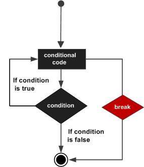
breakstatement to exit the loop when the mean ofSepal.Lengthis greater than 5. - Use
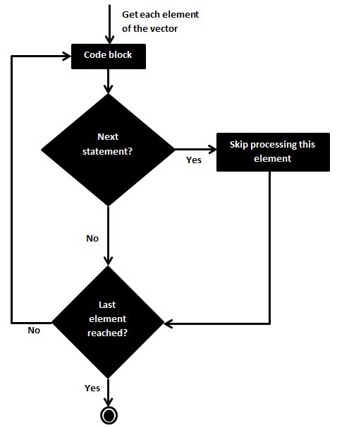
nextstatement to skip the iteration when the mean ofSepal.Lengthis less than 5.
- Use
- Use
applyfamily functions to calculate the mean, median, standard deviation, and standard error ofSepal.LengthandSepal.Widthfor each species in the new dataset.- Use boxplots for
Sepal.LengthandSepal.Widthfor each species in the new dataset.
- Use boxplots for
- Use the
cut()function to create a vector of intervals for each of the four floral traits (see?cut). Then, for each trait, make a contingency table of Species versus the interval factor of that trait, and draw a barplot of this table. In the barplot, there should be one bar per trait interval, with the counts of each species in this interval stacked. Combine the plots for the 4 floral traits into one plot, usinglayout().
![]()